Healy is getting a brand-spanking-new multibeam: an EM122!
Check out Dale Chayes' photo album of the replacement here. The pictures of them cutting into the hull are pretty sweet!

Thursday, December 3, 2009
Wednesday, December 2, 2009
Robot Clam to Detonate Underwater Mines!
I think this is really cool. My master's project involved using multibeam sonar to observe scour and burial of mines on the seafloor. It is a very real danger for ships going into some foreign waters. If this provides a safe means of detonation, then that is awesome!
http://www.livescience.com/technology/091201-robot-clam.html
http://www.livescience.com/technology/091201-robot-clam.html
Wednesday, November 25, 2009
Accent marks in JabRef
I have a lot of PDFs with authors that have accent marks in their names, such as Ekström. I had thought that using the LaTeX code for the letter in my JabRef entries might work since the database is just a BibTex file. No such luck. Turns out you can just use the regular keyboard shortcuts for Mac/Win in JabRef to get the right letters. For a guide to the keyboard shortcuts, check out this about.com link.
JabRef might complain about not being able to encode certain characters when you go to save your database. If so, just chose UTF-8 for the character encoding option. UTF-8 will preserve any letters with accents, as well as foreign characters you might have (e.g. Greek letters in the abstracts).
JabRef might complain about not being able to encode certain characters when you go to save your database. If so, just chose UTF-8 for the character encoding option. UTF-8 will preserve any letters with accents, as well as foreign characters you might have (e.g. Greek letters in the abstracts).
Zotero AND JabRef: how to make both work for you
So yesterday I posted about how I switched over to JabRef reference software, mainly because it allows relative links, but also because it easily lets you see and edit the BibTex entry, which as a LaTeX user, is very helpful. There are two things JabRef does not really do that Zotero does that I find really useful:
1) Zotero can easily capture reference information from a variety of website formats, even if no Bibtex or RIS entry is provided
2) You can drop a pdf directly into Zotero, index it, and then retrieve the reference information automatically, assuming the article is online somewhere
If the article's webpage has a BibTex or RIS entry available for download, you can simply download this and import it into your JabRef database, but I have noticed some journals still do not offer this service (shame on them!)
So this morning I have been happily using Zotero to collect reference information I find online and to auto-generate some entries based off some PDFs I already had. Once I am done, I can export to a RIS file and then import that RIS file to my current JabRef database. My BibTex keys are automatically generated on import, so I simply select the new entries, go to Tools -> Scan Database -> Sync Files and any new PDFs I obtained during the day will be linked to their entry in JabRef.
I keep my Main.bib file that is my current JabRef database inside my folder with all my reference PDFs. At the end of the day, I can simply commit the whole folder to subversion. Everything is not only backed up, but when I checked out the folder on my Windows machine, all my PDF links will work perfectly and I won't have to tweak my database one bit!
I used to hesitate putting all my PDFs in svn, but our school server is pretty huge and the 1 GB or so of PDFs that I have now does not even make a dent. Plus, after hearing from a friend how he lost his whole PDF database and had to go download or even scan (yikes!) all his references again, I decided backing up all my articles in svn was not only OK, but necessary!
Tuesday, November 24, 2009
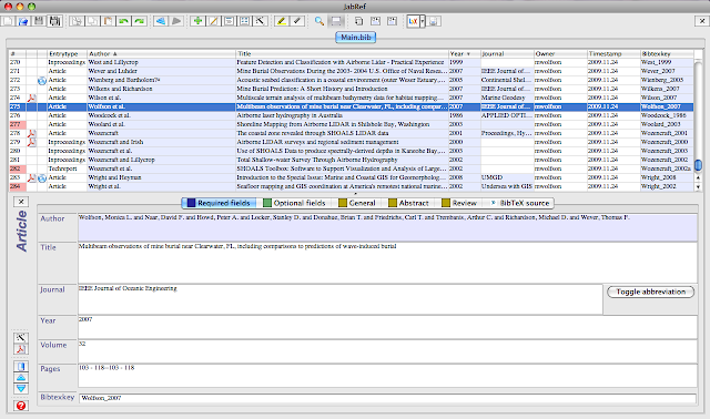
Zotero to JabRef: switching reference software
If you know the academic me, you know I love, and regularly tout, using Zotero to manage my ever-growing bibliography. There is one problem with Zotero, however, that I just cannot move past: its inability to use relative links for linking to files.
update: I edited the following paragraph to clear up some confusion pointed out in a posted comment. I should also point out that on Zotero's website, there are numerous posts from users requesting relative links, but with absolutely no reply from Zotero. This again makes me think that the way Zotero is written, relative links are not possible. Otherwise, they would have it, wouldn't they?
I love being able to sync my Zotero database between my personal Mac and school PC, but the syncing breaks the file links. If you sync your database to a second computer, it shows the links as still being there, but if you try to click on a file to open it within Zotero you get an error message saying Zotero cannot find it. You can tell Zotero where the file is, but you would have to do this for every file in the database. I am guessing this has something to do with Zotero running as a FireFox plug-in. When you add a PDF from another directory, Zotero copies it into its own internal structure, which is confusing and involves folders with random letter names. This is just not working for me. I want to be able to sync my database between my computers, and have functional links to the associated files.
I just switched today to JabRef and love it. It is free, works on Windows, Linux, and Mac, and let's you use relative links. It is simply a frontend for your BibTex file, but it has some really cool tricks:
1. It can autogenerate bibtex keys based on a format you specify
2. It can automatically link entries to files in any directory you specify based on the bibtex keys.
3. It is all stored in a small, easily transferable, BibTex file
4. It supports online searches so you can find and easily capture references online
5. It supports field-based views, but let's you view and directly edit the BibTex code as well as
4. I am sure there are a ton more, but I just started using it today
There are a couple tricks to switching over, so here is what I did:
1. Export the Zotero library in RIS format (my BibTex format export from Zotero caused issues with JabRef)
2. Import the RIS file into a new database in JabRef and save it
3. The internal PDF links from Zotero were written out to the URL field, meaning there are now a bunch of broken URL links in JabRef. To fix this, I navigated to the location of my new database file via terminal (or Cygwin in Windows) and did the following:
egrep -v "internal-pdf" original.bib > new.bib
This will delete all those pesky broken URLs that think they are internal PDF links, but still keep any legit URL links
4. Open the new.bib with JabRef (you can close out the old database now).
5. Under Options -> Preferences -> External Programs: Set the file and PDF directories to whatever directories you are already using (ex: /Users/mwolfson/Documents/School/Articles). Also check the "Autolink files with names starting with BibTex Key" option
6. Under the BibTex Key generator options, setup your BibTex key to match how you name your PDFs. My PDFs are named: author_year.pdf. So my BibTex Keys were set to [auth]_[year].
7. Select all your entries in your database, then go to Tools -> autogenerate BibTex Keys (let it overwrite old keys if necessary). Now all your entries should have the proper BibTex Key appended to them
8. While still selecting all records, Tools -> Scan Database -> Synchronize File Links (they have a specific PDF link, which works, but does not add the PDF icon to the entries for some reason -- perhaps because it uses a special pdf = {} in the bibtex code instead of file = {} -- so there is no way to know which entries have PDFs and which don't). Allow overwriting and hit OK. Now, if your PDF/file names in the specified directory match any of the BibTex keys, they will be auto-linked to the JabRef entry. Entries with linked PDFs should now show a PDF icon next to it.
update: There is an option under preferences to "show PDF/PS column" which would then, in fact, display the PDF icon if you choose to PDF sync rather than File sync. I have heard PDF/PS sync is being phased out since File sync handles these file types and more though, so I still recommend using File sync instead.
Viola! You should now have a working BibTex database in JabRef with all your articles linked. If you work across multiple computers like me, simply open up this database in JabRef on the new machine, set up your file directories to point to the appropriate files, and you are done. All your PDF links will work because the links themselves are relative! This is especially awesome when working cross-platform between Windows, Linux, and Mac.
Here is a screen grab showing what JabRef looks like running on my Mac:
If you get stuck feel free to drop me a comment and I'll try to help.
update: I edited the following paragraph to clear up some confusion pointed out in a posted comment. I should also point out that on Zotero's website, there are numerous posts from users requesting relative links, but with absolutely no reply from Zotero. This again makes me think that the way Zotero is written, relative links are not possible. Otherwise, they would have it, wouldn't they?
I love being able to sync my Zotero database between my personal Mac and school PC, but the syncing breaks the file links. If you sync your database to a second computer, it shows the links as still being there, but if you try to click on a file to open it within Zotero you get an error message saying Zotero cannot find it. You can tell Zotero where the file is, but you would have to do this for every file in the database. I am guessing this has something to do with Zotero running as a FireFox plug-in. When you add a PDF from another directory, Zotero copies it into its own internal structure, which is confusing and involves folders with random letter names. This is just not working for me. I want to be able to sync my database between my computers, and have functional links to the associated files.
I just switched today to JabRef and love it. It is free, works on Windows, Linux, and Mac, and let's you use relative links. It is simply a frontend for your BibTex file, but it has some really cool tricks:
1. It can autogenerate bibtex keys based on a format you specify
2. It can automatically link entries to files in any directory you specify based on the bibtex keys.
3. It is all stored in a small, easily transferable, BibTex file
4. It supports online searches so you can find and easily capture references online
5. It supports field-based views, but let's you view and directly edit the BibTex code as well as
4. I am sure there are a ton more, but I just started using it today
There are a couple tricks to switching over, so here is what I did:
1. Export the Zotero library in RIS format (my BibTex format export from Zotero caused issues with JabRef)
2. Import the RIS file into a new database in JabRef and save it
3. The internal PDF links from Zotero were written out to the URL field, meaning there are now a bunch of broken URL links in JabRef. To fix this, I navigated to the location of my new database file via terminal (or Cygwin in Windows) and did the following:
egrep -v "internal-pdf" original.bib > new.bib
This will delete all those pesky broken URLs that think they are internal PDF links, but still keep any legit URL links
4. Open the new.bib with JabRef (you can close out the old database now).
5. Under Options -> Preferences -> External Programs: Set the file and PDF directories to whatever directories you are already using (ex: /Users/mwolfson/Documents/School/Articles). Also check the "Autolink files with names starting with BibTex Key" option
6. Under the BibTex Key generator options, setup your BibTex key to match how you name your PDFs. My PDFs are named: author_year.pdf. So my BibTex Keys were set to [auth]_[year].
7. Select all your entries in your database, then go to Tools -> autogenerate BibTex Keys (let it overwrite old keys if necessary). Now all your entries should have the proper BibTex Key appended to them
8. While still selecting all records, Tools -> Scan Database -> Synchronize File Links (they have a specific PDF link, which works, but does not add the PDF icon to the entries for some reason -- perhaps because it uses a special pdf = {} in the bibtex code instead of file = {} -- so there is no way to know which entries have PDFs and which don't). Allow overwriting and hit OK. Now, if your PDF/file names in the specified directory match any of the BibTex keys, they will be auto-linked to the JabRef entry. Entries with linked PDFs should now show a PDF icon next to it.
update: There is an option under preferences to "show PDF/PS column" which would then, in fact, display the PDF icon if you choose to PDF sync rather than File sync. I have heard PDF/PS sync is being phased out since File sync handles these file types and more though, so I still recommend using File sync instead.
Viola! You should now have a working BibTex database in JabRef with all your articles linked. If you work across multiple computers like me, simply open up this database in JabRef on the new machine, set up your file directories to point to the appropriate files, and you are done. All your PDF links will work because the links themselves are relative! This is especially awesome when working cross-platform between Windows, Linux, and Mac.
Here is a screen grab showing what JabRef looks like running on my Mac:

If you get stuck feel free to drop me a comment and I'll try to help.
Monday, November 2, 2009
Installing GMT under Cygwin
I just struggled through installing GMT under Cygwin, and since I not only had to rely on piecing together information from out-of-date online tutorials, but also on direct help from Kurt, I figured I would write everything down here for future reference and to also hopefully make someone else's life easier.
First things first, check your home directory:
Always check your home directory in cygwin to see if it is actually what it should be. When you install Fledermaus on your machine, it sets a 'HOME' variable that is Program File/IVS/Fledermaus. Now Cygwin thinks this is its home as well. The CCOM wiki offers this solution:
To resolve this, you can create a system-wide HOME area that may be more suitable for any/all programs. To do this, create (or decide) the folder you'd like to be your Cygwin home area. Once you have the folder, edit the HOME variable in the Advanced System properties in Windows and specify that folder. Finally, copy the contents of the previously specified home area into your new home area folder. This will prevent IVS or GMT from breaking. This situation may not be limited to these two products, so it's important to check your 'HOME' environment variable before installing Cygwin software.
Once you are happy with your home directory, here are the steps I followed to successfully install GMT:
1) Make sure you have bzip2 installed. You will also need the 'make' utility and a good C++ compiler (I have a couple different ones, including the gcc one. netcdf will fail to compile without the right one, so if it fails, try grabbing another C compiler. I think gcc is the one to have).
2) Go to the GMT webpage and create an install parameter file. Save this as GMTparams.txt in your usr/local/ directory under your cygwin directory. (If you do not have netcdf already, make sure to let GMT get it and install it for you)
3) Get the GMT install file here, and save it as install_gmt to usr/local/
4) Under cygwin, navigate to usr/local/ and type the following command (this may fail, but this is okay):
./install_gmt GMTparams.txt > install.log
5) If it failed, you probably got a message about a missing -lnetcdf file. This is because netcdf is bad, and uses a .lib extension rather than .a. To fix this, you can just create a symbolic link:
navigate to usr/local/netcdf-xxx/lib
type ln -s libnetcdf.lib libnetcdf.a
Now modify your GMTparams.txt so that netcdf is not downloaded or installed again. You can also modify not to download the GMT files again.
6) navigate back to usr/local/ and rerun ./install_gmt GMTparams.txt >install.log. This should complete without failing, though you may see warnings scroll by.
7) Once it is installed, you must edit your .bashrc or .bash_profile. Cygwin, by default, does not create a .bashrc or .bash_profile in your home directory, so you may need to create one from scratch. GMT looks for a .bash_profile, so if you use .bashrc, make sure you create a .bash_profile that points to it. I'll share mine below:
my .bashrc file (all are needed for GMT to work):
export PATH=/usr/local/gmt/bin:$PATH
export NETCDFHOME=/usr/local/netcdf
export GMTHOME=/usr/local/gmt
export MANPATH=/usr/local/gmt/man:$MANPATH
export DISPLAY=:0
my .bash_profile file:
if [ -f ~/.bashrc ]; then
. ~/.bashrc
fi
export BASH_ENV=$HOME/.bashrc
8) Now you may notice that my paths in .bashrc do not seem to be correct. I use "gmt" and "netcdf" instead of "GMT4.5.1" and "netcdf-3.6.3." This is because I want to be able to update both of these in the future without having to edit any scripts or my .bashrc every time. Therefore I set up the following symbolic links:
navigate to usr/local/ and then type the following commands:
ln -s GMT4.5.1 gmt
ln -s netcdf-3.6.3 netcdf
9) You should be good to go!
To test one of the examples GMT runs upon successful install, you can navigate to any one of the examples found in /GMT4.5.1/share/doc/gmt/examples/. Each ex directory will contain the example scripts, necessary files, and the resulting postscript. I found that to view these files, I need to make sure the X-windows environment is up and running (from cygwin command prompt, type startx). Then I use ghostview (gs) to view the ps:
gs example_27.ps
here is the result:

Fun with Apple Terminal
I am starting to do more and more stuff on my Mac via the Apple Terminal, so I decided to spruce mine up a bit.
Using Fink I first installed "fortune-mod" (the program that actually displays the fortunes) and then installed "fortunes" (the fortunes themselves).
Next I simply added "/sw/bin/fortune" to my .bashrc file.
Now, whenever I open a new terminal window, I am greeted with a fun fortune. Most of the time, these seem to be just silly sayings, such as this:
Old programmers never die, they just become managers.
but every now and then you get something unexpected, such as a recipe for Glogg (a traditional Scandinavian holiday drink).
Tuesday, October 20, 2009
AGU recently announced a special late-breaking session for the fall meeting this year. Abstract deadline is Oct. 30th. This session is sure to be full of some exciting talks!
The 2009 Samoan and Sumatran Earthquakes: Origins, Impacts and Consequences
Category: Seismology
Co-Sponsors: G, NG, NH, OS, DI, T
On 29 September 2009 the Pacific plate ruptured in a normal faulting earthquake of magnitude 8.3 close to its subduction beneath the Australian plate. The resulting sea-floor displacement generated a tsunami that resulted in loss of life and great destruction in Samoa and American Samoa. Less than 20 hours later and some 10000 great circle kilometres distant a magnitude 7.6 event shook the city of Padang in Sumatra. At the time of writing over 1100 are confirmed dead, many more are still missing and great areas of the city are devastated. One day later another earthquake M6.6 ruptured the great Sumatran fault more than 250 km to the southeast.
Many important questions arise from these events: What was their mechanism and tectonic context?
What were the features of the Samoan event which generated the tsunami and how could its effect have been mitigated? Why was the Padang earthquake so devastating and what was its relationship to the recent great megathrust earthquakes on the Sunda subduction zone? What are the implications of this event for the high seismic and tsunami risk from near-future megathrust earthquakes west of Sumatra? How can we best prepare vulnerable populations for them? Finally, is the temporal clustering of these large events purely coincidence or if not, what physical mechanisms might explain it? We encourage submissions on all aspects of these earthquakes.
Tuesday, October 6, 2009
From GeoMapApp to Google Earth: Visualize your data in a jiffy!
Seriously!
I am not sure if the old version of GeoMapApp supported such an easy import/export of data, but the new version, released October 1, sure does!
Here is how to bring in your data, view it, color and scale by value, and export it to Google Earth in a jiffy. A jiffy, of course, being relative to the amount of data you actually have.
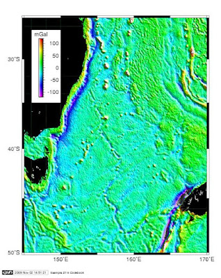
1) Under the File menu, import your data into GeoMapApp. This can be a shapefile, a 2D grid, or a table/spreadsheet in ASCII or Excel. I selected an Excel file of oceanic transform fault data and it worked flawlessly.
2) Once loaded, your data should display on the map and the data table will appear below. On the right you will notice several options related to the data table, including Color by Value and Scale by Value. Selecting these brings up a drop down box of all your data parameters. Select one and a color bar will pop up that you can edit. Once done, be careful not to close out the colorbar box or you will lose your settings (perhaps a bug? I simply minimize it to get it out of the way).
Here is what the transform fault data look like, colored by slip rate and sized by length:
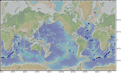
3) To export to Google Earth simply click on the save drop-down box on the right and select Export to Google Earth (KMZ). You can either export selected data points or your entire table. Once you make your selection, a box pops that enables you to select which parameters to export. The next step lets you choose what parameter the placemark name will take, as well as rename parameters and set units. Once you click okay, GeoMapApp will export the kmz file.
Here is my exported kmz file inside Google Earth:
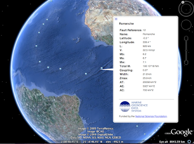
It does not color the placemarks by the value you selected in GeoMapApp, nor does it allow you to select your icon, but these things can be edited in the kmz file itself. What it does do is provide an easy way to get the data into Google Earth to begin with. Simply click on a placemark, and all your parameters for that point pop up!
So there you have it! Quick and easy data visualization in two great (and free!) geospatial data applications!
I am not sure if the old version of GeoMapApp supported such an easy import/export of data, but the new version, released October 1, sure does!
Here is how to bring in your data, view it, color and scale by value, and export it to Google Earth in a jiffy. A jiffy, of course, being relative to the amount of data you actually have.
1) Under the File menu, import your data into GeoMapApp. This can be a shapefile, a 2D grid, or a table/spreadsheet in ASCII or Excel. I selected an Excel file of oceanic transform fault data and it worked flawlessly.
2) Once loaded, your data should display on the map and the data table will appear below. On the right you will notice several options related to the data table, including Color by Value and Scale by Value. Selecting these brings up a drop down box of all your data parameters. Select one and a color bar will pop up that you can edit. Once done, be careful not to close out the colorbar box or you will lose your settings (perhaps a bug? I simply minimize it to get it out of the way).
Here is what the transform fault data look like, colored by slip rate and sized by length:

3) To export to Google Earth simply click on the save drop-down box on the right and select Export to Google Earth (KMZ). You can either export selected data points or your entire table. Once you make your selection, a box pops that enables you to select which parameters to export. The next step lets you choose what parameter the placemark name will take, as well as rename parameters and set units. Once you click okay, GeoMapApp will export the kmz file.
Here is my exported kmz file inside Google Earth:

It does not color the placemarks by the value you selected in GeoMapApp, nor does it allow you to select your icon, but these things can be edited in the kmz file itself. What it does do is provide an easy way to get the data into Google Earth to begin with. Simply click on a placemark, and all your parameters for that point pop up!
So there you have it! Quick and easy data visualization in two great (and free!) geospatial data applications!
Glossaries package in Texnic Center on Windows
Okay, yesterday I posted about how to set up and use the glossaries package with TexShop on a Mac. Here is the Windows version using TexnicCenter. This is basically a condensed version of Nicole Talbot's (creator of the glossaries package) post on the same matter:
If your TexnicCenter frontend is using the MikTex tex distribution, you can use the MikTix package browser to install packages (very easy to do, and the recommended method.) Otherwise you can install them manually from CTAN.
Using your preferred method, install the following packages:
* ifthen
* xkeyval at least version 2.5f (2006/11/18)
* xfor
* amsgen (part of amstex)
Make sure you have the following in your preamble:
\usepackage[acronym]{glossaries}%makes a separate acronym list
\makeglossaries
If you want your terms in your text to be hyperlinked to their definition (way cool), add the following BEFORE \usepackage{glossaries}:
\usepackage[colorlinks]{hyperref}
Now, as mentioned in the yesterday's post, you can either define terms and acronyms in your preamble, or have them as separate tex files and use the \include{} command.
When you get to the location in your main document (after the \begin{document}) where you want your glossary to be, simply add the command:
\printglossaries
Now, here is where it can get a bit tricky. You need to build the glossary file first, and there really isn't an easy way to simply add an engine to TexnicCenter (at least not that I found). Glossaries uses a Perl script to build, so I found the easiest way to do this is to make sure I have Perl installed on my machine (recommend Active Perl, they have windows installers). There are other ways to build the file using makeindex or xindy commands (see Nicola's post, but you have to run them 3 times for every type of glossary file, and the Perl way is just easier and faster.
Once you are good to go with Perl installed, open a command prompt (start->run->cmd) and navigate to the directory with your Tex files.
Type the following at the command prompt (you do not need to include a filename extension):
makeglossaries filename
You should see a bunch of stuff fly by on the screen indicating your glossary file was created. Now simply go back to TexnicCenter and build the file as you normally would, and Viola!, you should have a document with a glossary file.
Monday, October 5, 2009
Creating Glossaries in TexShop on Mac
I was searching for a way to create a word list or dictionary in Latex, and came across the Glossaries package. This package is already installed if you use TexShop for Mac, but I still had problems getting it to work.
The problem is that you first have to be able to build the glossary file before you build your main latex document (similar to when you create a bibliography using Bibtex).
I found a very helpful blog post about all this here: http://www.ict-cloud.ch/2009/07/glossaries-acronyms-and-texshop.html.
I followed his steps and created a text file called "glossary_run.engine" that contained the following code:
Save this file (you must use the .engine extension) to Users/.../Library/TexShop/Engines directory.
(Note: I first tried this with TextEdit. Even if you remove the .rtf extension, this will not work. It will work if you copy and paste the code into Emacs and then save it)
Next, make the file executable. In terminal, navigate to the above directory and type
$ chmod a+x glossary_run.engine
There you have it. The next time you open TexShop, the glossary_run engine (or whatever you named it) will be in the dropdown list next to typeset. Before you build your latex document, select this engine from the drop down and click typeset to build your glossary file first.
To use the glossaries package you will need the following in your preamble:
\usepackage[acronym]{glossaries} %makes a separate acronym list
%there are lots of different options for this package. acronym enables me to define acronyms as well as words
\makeglossaries
%Glossary-File - can include a separate glossary file here
\include{glossary file name.tex}
%Acronyms - can include a separate acronym file
\include{acronym file name.tex}
\begin{document}
Here is the test code I played around with. Instead of including separate files, I defined some terms and acronyms in the preamble. If I do it this way, I do not need the include terms, and instead just use the makeglossaries command:
\documentclass{article}
\usepackage[colorlinks]{hyperref}
\usepackage[acronym]{glossaries} % make a separate list of acronyms
\makeglossaries
%new glossary term
\newglossaryentry{sample}{name={sample}, description={a sample entry}}
%new acronym
\newacronym[\glsshortpluralkey=cas,\glslongpluralkey=contrived acronyms]{aca}{aca}{a contrived acronym}
\begin{document}
A \gls{sample} entry and %\gls{aca}.
Second use: \gls{aca}.
Plurals: \glspl{sample}.
%Reset acronym to first count
\glsreset{aca}
%note this now uses the plural form
First use: \glspl{aca}. Second use: \glspl{aca}.
\printglossaries
\end{document}
The problem is that you first have to be able to build the glossary file before you build your main latex document (similar to when you create a bibliography using Bibtex).
I found a very helpful blog post about all this here: http://www.ict-cloud.ch/2009/07/glossaries-acronyms-and-texshop.html.
I followed his steps and created a text file called "glossary_run.engine" that contained the following code:
#!/bin/sh

bfname=$(dirname "$1")/"`basename "$1" .tex`"

makeindex -s "$bfname".ist -t "$bfname".alg -o "$bfname".acr "$bfname".acn
makeindex -s "$bfname".ist -t "$bfname".glg -o "$bfname".gls "$bfname".glo
Save this file (you must use the .engine extension) to Users/.../Library/TexShop/Engines directory.
(Note: I first tried this with TextEdit. Even if you remove the .rtf extension, this will not work. It will work if you copy and paste the code into Emacs and then save it)
Next, make the file executable. In terminal, navigate to the above directory and type
$ chmod a+x glossary_run.engine
There you have it. The next time you open TexShop, the glossary_run engine (or whatever you named it) will be in the dropdown list next to typeset. Before you build your latex document, select this engine from the drop down and click typeset to build your glossary file first.
To use the glossaries package you will need the following in your preamble:
\usepackage[acronym]{glossaries} %makes a separate acronym list
%there are lots of different options for this package. acronym enables me to define acronyms as well as words
\makeglossaries
%Glossary-File - can include a separate glossary file here
\include{glossary file name.tex}
%Acronyms - can include a separate acronym file
\include{acronym file name.tex}
\begin{document}
Here is the test code I played around with. Instead of including separate files, I defined some terms and acronyms in the preamble. If I do it this way, I do not need the include terms, and instead just use the makeglossaries command:
\documentclass{article}
\usepackage[colorlinks]{hyperref}
\usepackage[acronym]{glossaries} % make a separate list of acronyms
\makeglossaries
%new glossary term
\newglossaryentry{sample}{name={sample}, description={a sample entry}}
%new acronym
\newacronym[\glsshortpluralkey=cas,\glslongpluralkey=contrived acronyms]{aca}{aca}{a contrived acronym}
\begin{document}
A \gls{sample} entry and %\gls{aca}.
Second use: \gls{aca}.
Plurals: \glspl{sample}.
%Reset acronym to first count
\glsreset{aca}
%note this now uses the plural form
First use: \glspl{aca}. Second use: \glspl{aca}.
\printglossaries
\end{document}
Yum! A nice, hot cup of putresince!
I suggest reading this with a nice hot mug of coffee by your side, as I did:
What's inside a cup of coffee?
What's inside a cup of coffee?
Tuesday, September 22, 2009
Leaf Peepers Report 2009!
New Hampshire maintains a foliage report website. It's pretty cool actually. Now I know that the leaves should still be turning when my folks are here in October. Check out the website for yourself here: http://foliage.visitnh.gov.ns1www.silvertech.net/index-flash.html


Sunday, September 20, 2009
Northeast Passage Navigible Once Again!
Two German tankers just became the first two Western ships to ever transit through the Northeast Passage!
http://news.bbc.co.uk/2/hi/europe/8264345.stm
http://news.bbc.co.uk/2/hi/europe/8264345.stm
Monday, August 31, 2009
A Call for Generic Sensor Format (GSF) files
I am putting out a call for GSF files to help test out the GSF-reader I am writing.
I have tested my GSF-reader with files I have found around CCOM; however, they all seem to be generated by CARIS, which only outputs certain records within the GSF file.
I am particularly interested in GSF files containing one or all of the following records:
1) BRB Intensity subrecord with time-series intensity records for each beam
2) Simrad, or non-Reson, sonar-specific subrecords
3) Sector Number, and Detection Info subrecord arrays
4) Reson-specific Quality Flags array
5) HV Navigation Error record
If you have such a GSF file that you can send me, please email me.
Cheers!
Thursday, August 27, 2009
Installing a Zagg Invisishield on iPhone 3G
I am posting this because a lot of people have posted about how hard it is to install a Zagg InvisibleShield on the iPhone 3G. I just put mine on and found it to be relatively easy, so I thought I would share a few tips in case it benefits anyone else.
1) Some folks complain that for best results you have to leave the phone off so it can "set up" for 12 to 24 hours to let the product cure. I simply installed mine at night so it can do most of its setting up while I am asleep.
2) Use the shield spray liberally! I ended up using the entire bottle just putting on the back piece because I had to realign it once and I wanted to keep my fingers moist. You can refill the bottle up to three times, so do not worry if you use a lot.
3) The corner pieces, were indeed, somewhat hard to do. They sort of stuck where they fell when I first placed the piece on the phone, so I had to peel them up, respray, and then press down again. Letting them set up a bit definitely helps as does the "palming method".
4) THE BEST ADVICE I found online was to stretch a piece of saran wrap over the top and bottom of the phone to help keep the corner pieces down while it cures. I did this for about 10 - 15 minutes only as I did not want to trap any moisture from the spray, but it did make a difference. My corners are all now nice and smooth.
The squeegee really did get most of the bubbles out, but some very small ones will remain. Zagg says these will work themselves out as the products settles down over the next day or two. I have been checking periodically as I let the phone sit, and indeed some of the small guys are already gone.
So far so good. I really like the shield and the phone looks great. I will still use my case for drop protection, but now I can rest assured about scratches.
I originally had an iFrogz Luxe case that I LOVED, until I realized it trapped stuff between the case and the phone, so the chrome and the back of the phone got scratched up a bit. I was always careful with the phone too, keeping it in a sunglasses pouch when in my purse, or keeping it in a separate pocket when in my book bag, so the scratches really annoyed me. Also, one of the tabs broke off after only a couple weeks, so I was worried about the case staying together if I were to drop the phone.
I now have a SwitchEasy Rebel. The case is not as nice looking or feeling as the iFrogz (in my opinion), but the protection seems to be way better and I am not worried about pieces snapping off.
Here are some pics of the phone about an hour and a half after putting on the Zagg:


UPDATE: Just FYI, by the next day, all micro-bubbles were gone, all the corners were smooth, and it looked awesome!
Follow Healy in Google Earth!
Thanks to Google and Kurt Schwehr, we can now follow Healy in Google Earth. Kurt's GeoRSS feed of the Healy's Aloftcon images is what is feeding the Google Earth visualization.
Check out Kurt's blog to see how to view it: Kurt's blog.
Check out Kurt's blog to see how to view it: Kurt's blog.
Wednesday, August 26, 2009
Healy Photostream on Flickr
The USCGC Healy has a photostream up on Flickr! Now we can all follow along as they traverse the Arctic! Check out the recently updated stream to see pics of a polar bear spotted just a couple days ago!
http://www.flickr.com/photos/cutterhealy/
http://www.flickr.com/photos/cutterhealy/
CARIS GSF: Update
So CARIS sure is speedy with their replies. I normally always hear back within a few hours, and sure enough, I had a response waiting for me this morning!
As with most programs that can write to GSF, CARIS simply implements the C-code available for download from SAIC's website. The extra-padding issue could be a bug in the original C-code then. Perhaps the 0 - 3 byte padding allowance listed in the specification document is not actually enforced.
However, I also wonder if this issue is related to the fact that CARIS only writes out sonar-specific sub-records for RESON systems. The GSFs I generate from RESON systems do not have the extra padding, but the SIMRAD ones do. I wonder if something about how the C-code writes out the records causes there to be extra bytes when the sonar sub-record it missing.
Maybe it is supposed to signify an unknown sonar type with an empty subrecord?
If someone happens to stumble along this post that has had a similar issue, feel free to drop me a line.
Tuesday, August 25, 2009
CARIS GSF and the Mysterious 2 Extra Bytes
I have been plowing along trying to get my GSF-reader I am coding up in Matlab to work with a variety of different GSF files (diff. versions as well as files from different GSF-generators). This morning I got my code to work with some CARIS-generated GSF files that were giving me a bit of a problem.
GSF records are often packed so that the total record size is an integral multiple of 4, so I wrote a little clean-up statement in all my sub-routines that will automatically read any extra characters needed to pad the particular record.
This one group of CARIS GSF files, however, keep crashing the reader. Within the Bathymetry Ping Record, I kept getting sub-record types of 0, which do not exist. I was at the end of the ping subrecords for the first ping in the file, and I had padded the record to be divisible by 4. The problem was that the total size of the ping record (including all sub-records) was 868 bytes, and even with the padding, I was only reading 864. Where were the extra two bytes coming from?
I ended up opening the GSF file itself and looking at it in Hex mode. This can be done using UltraEdit on Windows (automatically opens binary in Hex format) or by using AquaMacs on the Mac. I used ftell(fid) in Matlab to tell me where in the file I was when the error occurred and then went to that spot in the Hex mode file (in UltraEdit: Search -> GoTo line/Page and type in the number of bytes to move forward. in AquaMacs: C-u #bytes and then hit the right arrow key).
What I saw when I did this was that, sure enough, the record had extra padding. The total number of bytes in the ping sub-records for each ping is 862. To make this divisible by 4, you only have to add 2 bytes (thus my initial reading of 864 bytes). Looking at the binary in Hex mode, however, I was able to see that the record was actually padded with 6 bytes, bring the total up 868. Once I made this correction, the code ran happily and I was able to read the whole GSF file successfully.
I am still not sure what is up with the extra two bytes though, and I am curious to see if this may be the cause of GeoCoder and Fledermaus crashing when trying to read these files. I am going to submit this to CARIS and suggest they take a peak at it themselves. This bug only seems to occur in GSF files exported from CARIS 6.1 (I have tested it with different files). GSF files exported using CARIS 5.4 do not have the extra padding.
Monday, August 24, 2009
GSF-reader now working!!
Okay, so I am really excited because my GSF-reader that I coded up in Matlab is now working!! It is not fully-functional yet (I still have to add some sonar-specific readers, and some other optional record types) but it works for one of the sample CARIS-generated GSF files I have.
One of the things holding me up was the fact that I did not realize records were padded with extra bytes to ensure the record size in bytes was divisible by 4. I am not sure why it matters if it is divisible by 4, but apparently it does to GSF.
My next issue to tackle is a Reson sonar-specific quality flag indicator that is written in bits, not bytes, and uses all kinds of bit shifts and masks (joy!). This record is no longer used, but some older GSF versions will include them. Once that is tackled, some of the other GSF files should start working as well.
Also, if I want others to be able to benefit from this work, I should probably eventually convert it over to Python. Having a Python-based GSF reader would be pretty sweet.
There already exists C-code of course that does all this, but I want to have something that generates separate records for the data so that I can play with the ping depths for example, or the backscatter intensities, in a familiar environment. The C-code is really written so that it can be incorporated into other programs. By writing a reader myself, I not only gain a better understanding of the data and how GSF stores them, but I read them into a program where I can readily perform mathematical analysis on them.
Saturday, August 22, 2009
Methane Seeps from Arctic Seabed
Check out this discovery of deep-water methane seeps off Norway by a joint British-German research team:
http://news.bbc.co.uk/2/hi/science/nature/8205864.stm
below is a sonar image of some of the seeps

http://news.bbc.co.uk/2/hi/science/nature/8205864.stm
below is a sonar image of some of the seeps
Tuesday, August 18, 2009
Writing a GSF-reader in Matlab
I recently ran across a couple issues with some GSF (Generic Sensor Format) files I have, so I decided to attempt to write a GSF reader in order to see what, exactly, I was dealing with. I have never written any kind of binary format reader before (though I did tinker around and add features to one written in Python), so I sort of jumped in the deep-end with this. I decided to use Matlab, since I am most comfortable with its scripting language at this point in time.
Here is a valuable lesson I just learned: Never take the binary specification file at face-value. Typos happen, and they certainly happened here. I have the GSF v. 3.01 specification file available from the SAIC website, and have been following it to write my reader. Everything has been going fine for the most part until I reached the attitude record.
According to the specification, the attitude record should look like this:
-->
Should be pretty straightforward, so in my Matlab code I wrote the following function:
This returned all sorts of funky data that made no sense, most notably the negative times and pitch angles of 120 degrees (that would be worse than the perfect storm!). I decided to look at the GSF library also available on the SAIC website in order to check out the source code. In the library directory, there is a file called GSF_dec.c, a C-code source file for decoding the GSF binary format. I looked up how the Attitude record was decoded in C, and saw this:
>and a little farther down I saw:
The C-code shows that the specification table was completely wrong! There is only one reference time for the attitude reading, and the rest of the times are simply how many seconds past that reference time the rest of the measurements take place. Furthermore, the specifications stated that the Heave and Heading fields were text (something I thought was weird anyway) and in the C-code we clearly see they are integers. The specification also stated everything was 4-bytes, but it is actually only 2 (16 bits). This is very frustrating that the specification and the C-code do not match, especially since they both come from the same source.
At any rate, I am now able to write a working function that can be called in my main code:
Here is a valuable lesson I just learned: Never take the binary specification file at face-value. Typos happen, and they certainly happened here. I have the GSF v. 3.01 specification file available from the SAIC website, and have been following it to write my reader. Everything has been going fine for the most part until I reached the attitude record.
According to the specification, the attitude record should look like this:
-->
Field Name
|
Description
|
Field Type
|
Count
|
NUM_MEASUREMENTS
|
Number of attitude measurements in this record.
|
I
|
2
|
ATTITUDE_TIME
|
Array of attitude measurement times
|
I
|
N*2*4
|
PITCH
|
Array of pitch measurements
|
I
|
N*4
|
ROLL
|
Array of roll measurements
|
I
|
N*4
|
HEAVE
|
Array of heave measurements
|
T
|
N*4
|
HEADING
|
Array of heading measurements
|
T
|
N*4
|
Attitude Record Size:
|
Variable
| ||
Should be pretty straightforward, so in my Matlab code I wrote the following function:
function [Num_meas, ATT_Time, ATT_Pitch, ATT_Roll, ATT_Heave, ATT_Heading] = readATTrecord(fid)
%% This function reads the Attitude record in a GSF file.

%% Element          Bytes   Type         Description
% Num_Measurements    2      int      number of attitude measurements (N)
% Attitude_Time       N*2*4  int      array of attitude meas. times
% Pitch               N*4    int      array of pitch measurements (hundreths of deg)
% Roll                N*4    int      array of roll measurements (hundreths of deg)
% Heave               N*4    char      array of heave measurements (hundreths of deg)
% Heading             N*4    char      array of heading measurements (hundreths of deg)

Num_meas = fread(fid,1,'int16');

for i = 1:Num_meas
ATT_Time(i,:) = fread(fid,2,'int32');
end
for i = 1:Num_meas
ATT_Pitch(i,:) = fread(fid,1,'int32');
end
for i = 1:Num_meas
ATT_Roll(i,:) = fread(fid,1,'int32');
end
for i = 1:Num_meas
ATT_Heave(i,:) = fread(fid,4,'char');
end
for i = 1:Num_meas
ATT_Heading(i,:) = fread(fid,4,'char');
end
This returned all sorts of funky data that made no sense, most notably the negative times and pitch angles of 120 degrees (that would be worse than the perfect storm!). I decided to look at the GSF library also available on the SAIC website in order to check out the source code. In the library directory, there is a file called GSF_dec.c, a C-code source file for decoding the GSF binary format. I looked up how the Attitude record was decoded in C, and saw this:
gsfDecodeAttitude(gsfAttitude *attitude, GSF_FILE_TABLE *ft, unsigned char *sptr)
{
unsigned char *p = sptr;
gsfuLong ltemp;
gsfuShort stemp;
gsfsShort signed_short;
int i;
struct timespec basetime;
double time_offset;
/* First four byte integer contains the observation time seconds */
memcpy(<emp, p, 4);
p += 4;
basetime.tv_sec = ntohl(ltemp);
/* Next four byte integer contains the observation time nanoseconds */
memcpy(<emp, p, 4);
p += 4;
basetime.tv_nsec = ntohl(ltemp);
/* Next two byte integer contains the number of measurements in the record */
memcpy(&stemp, p, 2);
p += 2;
attitude->num_measurements = ntohs(stemp);
>and a little farther down I saw:
/* Now loop to decode the attitude measurements */
for (i = 0; i <>num_measurements; i++)
{
/* Next two byte integer contains the time offset */
memcpy(&stemp, p, 2);
time_offset = ((double) ntohs (stemp)) / 1000.0;
p += 2;

LocalAddTimes (&basetime, time_offset, &attitude->attitude_time[i]);

/* Next two byte integer contains the pitch */
memcpy(&stemp, p, 2);
signed_short = (signed) ntohs(stemp);
attitude->pitch[i] = ((double) signed_short) / 100.0;
p += 2;

/* Next two byte integer contains the roll */
memcpy(&stemp, p, 2);
signed_short = (signed) ntohs(stemp);
attitude->roll[i] = ((double) signed_short) / 100.0;
p += 2;

/* Next two byte integer contains the heave */
memcpy(&stemp, p, 2);
signed_short = (signed) ntohs(stemp);
attitude->heave[i] = ((double) signed_short) / 100.0;
p += 2;

/* Next two byte integer contains the heading */
memcpy(&stemp, p, 2);
attitude->heading[i] = ((double) ntohs(stemp)) / 100.0;
p += 2;
The C-code shows that the specification table was completely wrong! There is only one reference time for the attitude reading, and the rest of the times are simply how many seconds past that reference time the rest of the measurements take place. Furthermore, the specifications stated that the Heave and Heading fields were text (something I thought was weird anyway) and in the C-code we clearly see they are integers. The specification also stated everything was 4-bytes, but it is actually only 2 (16 bits). This is very frustrating that the specification and the C-code do not match, especially since they both come from the same source.
At any rate, I am now able to write a working function that can be called in my main code:
function [ATT_Time, Num_meas, ATT_Offset, ATT_Pitch, ATT_Roll, ATT_Heave, ATT_Heading] = readATTrecord(fid)
%% This function reads the Attitude record in a GSF file.

%% Element          Bytes   Type         Description
% ATT_Time            2*4    int      time of attitude meas.
% Num_Measurements    2      int      number of attitude measurements (N)
% Time_Offset         N*2    int      time offset in seconds
% Pitch               N*2    int      array of pitch measurements (hundreths of deg)
% Roll                N*2    int      array of roll measurements (hundreths of deg)
% Heave               N*2    int      array of heave measurements (hundreths of deg)
% Heading             N*2    unit     array of heading measurements (hundreths of deg)

ATT_Time = fread(fid,2,'int32');
Num_meas = fread(fid,1,'int16');

for i = 1:Num_meas
ATT_Offset(i,:) = fread(fid,1,'int16');
end
for i = 1:Num_meas
ATT_Pitch(i,:) = fread(fid,1,'int16');
end
for i = 1:Num_meas
ATT_Roll(i,:) = fread(fid,1,'int16');
end
for i = 1:Num_meas
ATT_Heave(i,:) = fread(fid,1,'int16');
end
for i = 1:Num_meas
ATT_Heading(i,:) = fread(fid,1,'uint16');
end
Sunday, August 2, 2009
Mobile Blog Photo Test

pic I snapped with my phone of a weird bug on my porch.
Mobile Blogging
So google blogger lets users blog on the go in a couple different ways. You can use SMS messaging (standard text messages), MMS messaging (multimedia messaging), or your email. Since I do not have a text plan, I opted for the latter. You set up an email address for your blog (under your existing blog's settings) and then just email your posts. You can select to have mobile posts immediately published or saved as drafts.
So here is my first post sent from my phone. I can also see this as a great way to blog from sea, when you often have email access but not full web capabilities.
So here is my first post sent from my phone. I can also see this as a great way to blog from sea, when you often have email access but not full web capabilities.
Importing Music into GarageBand and Making Ringtones
Okay, so I do not know about you, but I was somewhat annoyed to find out that not only will iTunes only let you create a ringtone from music you purchase from the iTunes Store, but that they still charge you an additional 99 cents to convert the song sample into ringtone format.
Total rip-off! Especially considering you already own the song!
Here's a free workaround: Kurt suggested that I try GarageBand, a music creation software that comes free with the Mac. It took a little futzing around, but I have now successfully (and freely) created a ringtone from Michael Jackson's The Way You Make Me Feel.
Here are the steps:
1) Open GarageBand and then drag-n-drop your music file (.mp3 works for sure, not sure about AAC) in it. The file should open right up as long as it is not DRM, so no purchases music from iTunes (though supposedly if you burn them to disc and then re-import, it loses the DRM)
2) Click on the scissors icon on the bottom left to bring up the track editor, and from there, click on the loop arrow icon to enable the loop feature. GarageBand ringtones are limited to loops of 40 seconds or less.
3) You should now see a second time bar appear just below the first at the top of the window (click the screen grab below to see what I am talking about). Just click and drag within the bar to select a portion of the song. The time bar will turn yellow where you select.
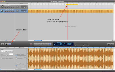
4) Just hit play to preview your selection. GarageBand will continuously loop through the selection, so you can get a pretty good idea of how your ringtone will sound.
5) Once you are happy with your selection, click on Share in the Menu Bar and select Send Ringtone to iTunes. It will convert the song for you and automatically open iTunes, where your song is stored in a new Ringtones folder. Now all you have to do is transfer it to your device.
Friday, July 31, 2009
A Bookstore and Free WiFi: Like Peanut Butter and Chocolate!
It's finally happened. Barnes and Nobles is now offering free WiFi in all their stores.
http://www.barnesandnoble.com/help/cds2.asp?r=1&PID=27206
One of my favorite combinations (outside peanut butter and chocolate) is a good bookstore (avec cafe) and free wifi.
http://www.barnesandnoble.com/help/cds2.asp?r=1&PID=27206
One of my favorite combinations (outside peanut butter and chocolate) is a good bookstore (avec cafe) and free wifi.
Tuesday, July 21, 2009
USGS Woods Hole: An Excellent Metadata Example!
Over the last couple years or so, I have become more and more concerned about metadata. Metadata is basically a file (txt, html, or xml) that accompanies a dataset and describes how, why, and when the data were collected, how they were processed, and who the primary contacts are. It can get more complicated, and there is also the matter of formats and whether or not it is compliant with the FGDC (Federal Geographic Data Committee) standards, but suffice to say the role of metadata is to give anyone reading it sufficient knowledge to be able to confidently use the data.
Good metadata is hard to find, and people routinely seem to underestimate its importance. Even if people do fill out metadata, they often skip a lot of important fields or simply do not include all the pertinent information (e.g. the tide station used to correct their data). What good is a multibeam dataset, for example, if I do not know how it was collected, if/how they corrected for tides and vessel motion, how they processed it, etc.? Oh sure, maybe you know what organization collected it, but what if they cannot remember? What if the main person responsible for that data no longer works there? A proper metadata file that accompanies the data will solve these issues.
Today I came across what I consider to be perhaps one of the best examples of metadata that I have seen. The metadata is for a multibeam dataset collected by the USGS in Woods Hole. All the pertinent fields are filled out, and for each section there is a point of contact listed. The reasons for the survey are given, as are the vessel used, the sonar used, how the sonar was mounted, etc. Not only did they specifically mention how they measured their vertical/horizontal accuracy and include an estimated uncertainty, but they include their tidal station information complete with NOAA tide station number so I can easily go and obtain the same tide record myself. What is most impressive, however, is that they list all their processing steps. They processed their data using SwathEd, a program developed at UNB that I am not familiar with. No problem though, because in the metadata, they actually give a numbered list of their processing steps complete with the command lines needed to do it myself! It is even broken up into editing that was done at sea, and the final editing steps undertaken to create the grids once they were back in the office.
Of course, no matter how good the metadata are, there is always room for some improvement. For example, it would be nice to see a separate ancillary data section perhaps, that lists the specific type and brand of IMU used, the type of CTD or sound velocimeter used, etc., along with manufacturer-stated (or observed) uncertainties.
Check out the USGS metadata, and of course the accompanying data, here: USGS Stellwagen Bank data. The data and metadata are all located under the GIS data links. The specific file I was looking at is here.
Here are some snippets of the metadata file to give you an idea (Note there are chunks of metadata skipped between snippets):
____________________________________________________
Good metadata is hard to find, and people routinely seem to underestimate its importance. Even if people do fill out metadata, they often skip a lot of important fields or simply do not include all the pertinent information (e.g. the tide station used to correct their data). What good is a multibeam dataset, for example, if I do not know how it was collected, if/how they corrected for tides and vessel motion, how they processed it, etc.? Oh sure, maybe you know what organization collected it, but what if they cannot remember? What if the main person responsible for that data no longer works there? A proper metadata file that accompanies the data will solve these issues.
Today I came across what I consider to be perhaps one of the best examples of metadata that I have seen. The metadata is for a multibeam dataset collected by the USGS in Woods Hole. All the pertinent fields are filled out, and for each section there is a point of contact listed. The reasons for the survey are given, as are the vessel used, the sonar used, how the sonar was mounted, etc. Not only did they specifically mention how they measured their vertical/horizontal accuracy and include an estimated uncertainty, but they include their tidal station information complete with NOAA tide station number so I can easily go and obtain the same tide record myself. What is most impressive, however, is that they list all their processing steps. They processed their data using SwathEd, a program developed at UNB that I am not familiar with. No problem though, because in the metadata, they actually give a numbered list of their processing steps complete with the command lines needed to do it myself! It is even broken up into editing that was done at sea, and the final editing steps undertaken to create the grids once they were back in the office.
Of course, no matter how good the metadata are, there is always room for some improvement. For example, it would be nice to see a separate ancillary data section perhaps, that lists the specific type and brand of IMU used, the type of CTD or sound velocimeter used, etc., along with manufacturer-stated (or observed) uncertainties.
Check out the USGS metadata, and of course the accompanying data, here: USGS Stellwagen Bank data. The data and metadata are all located under the GIS data links. The specific file I was looking at is here.
Here are some snippets of the metadata file to give you an idea (Note there are chunks of metadata skipped between snippets):
- Data_Quality_Information:
-
- Attribute_Accuracy:
-
- Attribute_Accuracy_Report: No attributes are associated with these data.
- Completeness_Report:
- These data were corrected for tidal elevation using the NOAA Boston tide gage. This assumes that the tidal elevation and phase are the same as Boston across the survey area. Further processing to correct for the spatial and temporal changes in tidal elevation across the survey area may be undertaken at a later time.
- Positional_Accuracy:
-
- Horizontal_Positional_Accuracy:
-
- Horizontal_Positional_Accuracy_Report:
- These data were navigated with a Differential Global Positioning System (DGPS); they are accurate to +/- 3 meters, horizontally.
- Vertical_Positional_Accuracy:
-
- Vertical_Positional_Accuracy_Report:
- These data have been corrected for vessel motion (roll, pitch, heave, yaw) and tidal offsets, and referenced to mean lower low water. The theoretical vertical resolution of the Simrad EM-1000 multibeam echosounder is 1 % of water depth, approximately 0.3 - 1.0 m within the study area.
____________________________________________________
- Process_Step:
-
- Process_Description:
- Data acquisition at sea
These multibeam data were collected with a Simrad EM1000 multibeam echo sounder mounted on the starboard pontoon of the Canadian Hydrographic Service Vessel Frederick G. Creed. The data were collected over four cruises carried out between the fall of 1994 and fall of 1998. Operation of the Simrad EM1000 was carried out by hydrographers of the Canadian Hydrographic Service. Data were collected along tracklines spaced 5-7 times the water depth apart at a speed of 10-14 knots. The frequency of the sonar was 95kHz. Sound velocity profiles were obtained and input into the Simrad processing system to correct for refraction. Navigation was by means of differential GPS.
- ____________________________________________________
- Process_Step:
-
- Process_Description:
- Final data processing and editing
Processing was carried out to further edit and correct the data and to produce final grids and images of the data. Processing and editing steps included:
1. Correct errors in soundings due to sound refraction, caused by variations in sound velocity profile, using the SwathEd refraction tool. These artifacts can be recognized in a cross-swath profile of a relatively flat patch of sea floor. When viewing the swath data across a profile, the sea floor will appear to have a "frown" or "smile" when in fact the data should be flat across the profile. Insufficient and/or erroneous sound velocity information, which is usually due to widely spaced or non-existent velocity profiles within an area, results in an under or over-estimate of water depth which increases with distance from the center of the swath. For a discussion of how this effect can be recognized in a swath bathymetric data file, see <
2. Remove erroneous soundings that were not edited in the field using the SwathEd program.
3. Correct the bathymetric data to mean lower low water by subtracting the observed tide at Boston, Massachusetts from the edited bathymetric soundings. This correction assumes that the tidal phase and amplitude are the same as Boston across the survey area.
Mean Lower Low Water (MLLW) tidal information was obtained from the NOAA tide server using tide station 8443970 located at Boston, MA (42 degrees 21.3 minutes N, 71 degrees 3.1 minutes W) (
Command line: binTide -year YYYY asciiTideFile BinaryTideFile
The program mergeTide brings the swath soundings to the MLLW vertical tidal datum:
Command line (tides): mergeTide -tide BinaryTideFile filename.merged Command line (navigation): mergeNav -ahead 5.379 -right 3.851 -below 4.244 filename (prefix only)
4. Create a 6-m grid of the bathymetric soundings for western Massachusetts Bay Quadrangles using the SwathEd routine weigh_grid.
Command line: weigh_grid -fresh_start -omg -tide -coeffs -mindep -2 -maxdep -800 -beam_mask -beam_weight -custom_weight EM1000_Weights -butter -power 2 -cutoff 12 -lambda 3 gridFile filename.merged
5. Convert binary bathymetric grid to ESRI ASCII raster format:
Command line: r4toASCII gridFile.r4
This creates a file called gridFile.asc.
Thursday, July 16, 2009
Image Processing in Matlab: Update 1: Filters
Okay, so I have been continuing to play around, trying to get my feet wet with image processing. I sort of jumped ahead here and begin fiddling with filters. Since I have the nadir artifact in my mosaic, I need to see if I can easily remove it.
I decided to use an adaptive filter since the noise I am most concerned is repetitive through the image (though not truly periodic as survey line spacing varies), so I do not need the same level of filtering over the whole image. I have been reading through the Matlab Image Processing documentation(pdf), and followed their directions for using "wiener2" which adaptively applies a Wiener linear filter to the image.
from the description under "help wiener2":
WIENER2 lowpass filters an intensity image that has been degraded by
constant power additive noise. WIENER2 uses a pixel-wise adaptive Wiener
method based on statistics estimated from a local neighborhood of each
pixel.
I used a 10x10 pixel neighborhood for filtering. Then, I ran the Sobel edge detect algorithm as described in my previous post. The results are below:
 on the left: orginal image on the right: wiener2 filtered image. Click to see full-size image so you can see the differences.
 The nadir artifacts are clearly less noticeable in the filtered image, and indeed the edge detect algorithm is now starting to pick up on the actual different patches of seafloor. The outline of the bright patch in the middle can now be seen.
I then increased the size of my filter to 20x20 pixels. Check out how well the edge detect performs now.


Beginning Image Processing in Matlab
I am starting to explore image processing in Matlab, and so far I am impressed with how easy it seems. I began with a 2000 x 2000 pixel gray scale image of a backscatter mosaic from EM3002 multibeam sonar data. I saved this image as a .tif and loaded it into Matlab using the 'imread' function. Once loaded, using "imshow" will display the image.
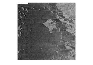
One of the first things I tried was the histogram function "imhist", to see how spread out my pixel values were between 0 - 255. Clearly my image does not make use of the full range of colors.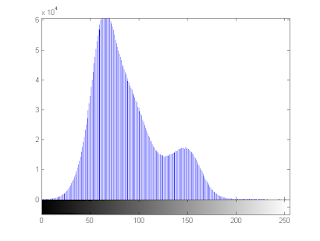 I then used "histeq" to stretch the intensity values between the full range of colors. Below are the resulting histogram and new higher contrast image.
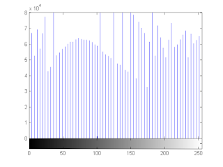
 You can clearly see the artifacts from the nadir beam of the sonar where you get a brighter return. I figured this would be a good test of one of the edge detect algorithms to see if it picks them all out. I used the "edge" command and specified the Sobel method, leaving the threshold value blank. You can also specify a direction, however, I left it as the default, which looks for both horizontal and vertical edges. Here are the results:
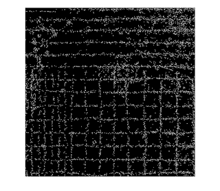 Pretty cool. It almost looks like a trackline map of the survey!

One of the first things I tried was the histogram function "imhist", to see how spread out my pixel values were between 0 - 255. Clearly my image does not make use of the full range of colors.
 I then used "histeq" to stretch the intensity values between the full range of colors. Below are the resulting histogram and new higher contrast image.
 You can clearly see the artifacts from the nadir beam of the sonar where you get a brighter return. I figured this would be a good test of one of the edge detect algorithms to see if it picks them all out. I used the "edge" command and specified the Sobel method, leaving the threshold value blank. You can also specify a direction, however, I left it as the default, which looks for both horizontal and vertical edges. Here are the results:
 Pretty cool. It almost looks like a trackline map of the survey!
Saturday, July 4, 2009
Daylilies in full bloom
After an exhausting roadtrip from KY back to NH, it was nice to come home and see the Daylilies in full bloom.

Blogger likes to resample the color scheme when it resizes the image to fit inside the blog post, so if you want to see the lilies in all their glory, be sure to click on the pic to see it full size:

Blogger likes to resample the color scheme when it resizes the image to fit inside the blog post, so if you want to see the lilies in all their glory, be sure to click on the pic to see it full size:
Wednesday, June 24, 2009
iPhone as a tool for hydrographers
So from Kurt's post on the iPhone as a tool for field geologists, and the subsequent posts he linked to, I began thinking about applications that I would like to see on an iPhone (not that I own one or anything) to help make it a handy little field tool for hydrographers. There are some pretty sweet hydro-licious applications for the iPhone that already exist (check out TideApp and iNavX), and I am sure this is only the beginning. Here are a couple of proposed apps of my own:
1) Equipment/Serial Number App:
Something like this may exist. It would be handy to have a little app that could organize lists of equipment and their serial numbers. Each entry could link to a picture of the object stored within the iPhone. Clicking on each entry would then bring up the picture, manufacturer, contact info for service/repair, a link to the website, and perhaps even a link to the online manual (or a PDF stored on the phone).
2) Ship Light App:
I am not sure if the flashlight app has this feature already or not, but having the screen emit a red light for night-safe vision on the ship instead of a bright white light would be excellent.
3) Vessel Offset App:
An app that could be used to generate a little diagram of the ship complete with vessel offsets between the transducers, IMU, etc. Perhaps it could sort of be a fill-in-the-blank type of program, so you know right away if you are missing a crucial value. This happened during my field course, and while I am sure seasoned hydrographers have much less of a chance of making this mistake, and if you always survey on the same ship it is probably not as necessary, I still think this would be pretty helpful. With this app, you could always have a copy with you that could be used for reference or could be emailed to someone else.
Thursday, June 11, 2009
M&M Mars: Free Chocolate Relief Act!
Tired of everyone getting stimulus packages but you? Well, M&M Mars is helping out by giving away free full-size chocolate bars every Friday through September. All you have to do is sign up every Friday morning, and within a couple weeks you will get a coupon for a free candy bar in the mail.
Check it out: https://secure.realchocolate.com/
Monday, June 8, 2009
Fugro to buy Tenix LADS
Fugro, one of the world's leading survey companies both on- and offshore, looks like they are about to acquire the Australian-based Tenix LADS Cooporation. Tenix LADS is one of the global providers of airborbe lidar bathymetry, and has completed many contracts under NOAA and the US Navy. Another one of Fugro's subsidies, Fugro Pelagos Inc., also conducts surveys for NOAA utilizing an Optech SHOALS-1000T lidar system.
Here is the full blurb at Hydro International: http://www.hydro-international.com/news/id3216-Fugro_Acquires_Tenix_LADS.html
Here is the full blurb at Hydro International: http://www.hydro-international.com/news/id3216-Fugro_Acquires_Tenix_LADS.html
Thursday, June 4, 2009
Seafloor Images of Air France Crash Site Available
CCOM/JHC has been putting together seafloor images to help aid in the search for Air France Flight 447
http://www.unh.edu/news/cj_nr/2009/june/bp4seafloor.cfm

http://www.unh.edu/news/cj_nr/2009/june/bp4seafloor.cfm

The Exploration of Challenger Deep
Man, I cannot even imagine the excitement and anticipation the scientists on this project must feel!!
Point Loma scientists on team taking vehicle to the deepest place on Earth
Posted using ShareThis
Point Loma scientists on team taking vehicle to the deepest place on Earth
Posted using ShareThis
Friday, May 29, 2009
Easy Tables in TexShop on a Mac
Okay, so while Excel2Latex works great on my PC at school, it does not work so hot on my Mac running Excel 2004. TexShop was not happy with the output code at all. I tried some tips I found online, but no luck. Then I came across:
Cal2LaTex for OpenOffice and NeoOffice. This tool works like a charm and its menu options are superior to that of Excel2Latex. It did take me a few minutes to figure out how to assign the Macro its own listing under my Tools menubar, but other than that getting it working was a breeze.
And let's face it, on a Mac at least, NeoOffice seems to run better than MS Office anyway. Of course, since I discovered LaTex I generally only ever open Word when I have to open someone else's document. :)
Tables in LaTex Made Easy!
Tables in Latex can be rather tricky, and I wanted to find some way of creating a table quickly that would look good. In Googling around, I stumbled across Excel2Latex. This little macros tool will add a toolbar button that will allow you to export directly from a table you have formatted in Excel (Mac or PC versions) into a piece of Latex code that can be pasted into you Tex document. Once in Tex, you can add some snazzy formatting (like lines, etc.) and you are all set. Excel2Latex will even convert all font formatting (bold, italic, etc.) for you.
Check out the results (I used /hline to add some lines to the original exported code):
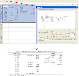
Note: I did have some troubles running the macros at first. I kept getting: "Error: Can't find project or library."
The Solution: Open your VBA editor in Excel (from Excel hit alt+F11) and then go to Tools -> References. Scroll down until you see the reference labeled MISSING and simply uncheck it.
The tool should now work.
Monday, May 25, 2009
Seamless land/sea mapping with Lidar
I am currently working up some Tenix LADS MKII lidar data over the Isles of Shoals off the coast of New Hampshire. I must say, the data set is quite impressive. Not only does the lidar bathymetry match very well with EM3002 multibeam bathymetry we have in the same area (initial comparison shows a mean difference of 0.6 m w/ a std: 0.3 m), but the seamless transition of the lidar data from water to land follows very closely the transition between the foreshore and the water (soundings are reduced to MLLW).
Here you can see the transition from depth soundings (blue) to terrain heights (brown) from the LADS lidar system. The flightlines are oriented north-northeast by south-southwest. NOAA chart 13283 is peeking out from behind the soundings. You can just see how the transition in sounding type roughly follows the foreshore line (MLLW) on the chart.
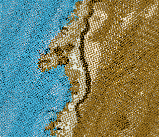
What does the bathymetry from the LADS MKII lidar look like? Here's a peak of some of the lidar bathy data (blue soundings only) gridded at a 4-meter resolution and displayed in Fledermaus. Sun illumination is from the northwest and the vertical exaggeration is 3. NOAA chart 13283 is in the background.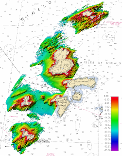

Friday, May 8, 2009
LIDAR view of the Golden Gate Bridge
The Seafloor Mapping Lab at the California State University in Monterey Bay has recently obtained a new vessel-mounted Lidar system for shoreline surveys. From their website:
Integration of this technology with their existing mapping systems allows for some pretty impressive data displays:
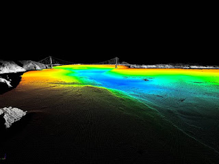 Combined bathy/topo DEM of the Golden Gate built by merging SFML's laser scanner (gray) and multibeam sonar (colored by depth) data (source: http://seafloor.csumb.edu/laserscanner.html)
They also have some pretty sweet 3D fly-throughs of the Golden Gate Bridge and the Los Padres Reservoir. I have included their Golden Gate Bridge fly-through below:
The high-resolution data set seen above was collected using SFML's new vessel-mounted mobile marine LIDAR system. Working with our industry partners, Riegl and Applanix, we have implemented an easily and rapidly deployable laser scanner capable of achieving decimeter accuracy with sub-meter resolution at a 1 kilometer range. This system gives SFML the ability to map the intertidal shoreline, offshore rocks and pinnacles and coastal features in unprecedented detail without the need for more costly airborne LIDAR surveys. The high spatial precision and accuracy of the system enable SFML to reliably monitor and quantify coastal erosion and landslide rates, bridge deformation, railway subsidence and coastal highway slippage through repetitive shoreline mapping surveys; information critical to coastal communities as they plan for climate change and sea level rise.
Integration of this technology with their existing mapping systems allows for some pretty impressive data displays:
 Combined bathy/topo DEM of the Golden Gate built by merging SFML's laser scanner (gray) and multibeam sonar (colored by depth) data (source: http://seafloor.csumb.edu/laserscanner.html)
They also have some pretty sweet 3D fly-throughs of the Golden Gate Bridge and the Los Padres Reservoir. I have included their Golden Gate Bridge fly-through below:
Subscribe to:
Posts (Atom)